As previous reports have indicated, there is widespread price variation in the U.S. commercial health care system. Many studies have shown that prices are dramatically different not only across geographies, but they vary substantially even within the same market for the same service. For example, we found that prices for the same blood tests could vary 39-fold within Tampa, Florida and the cost of a C-section delivery could vary by more than $24,000 in San Francisco, California, depending on the provider.
In response to this dramatic price variation, many Congressional, administrative, and state legislative activities have promoted the need for greater price transparency in health care. For instance, as of January 2019, the Centers for Medicare and Medicaid Services (CMS) required all hospitals make public their “current standard charges” online for consumers to access. Most recently, the Departments of Health and Human Services, Labor, and the Treasury issued a proposed rule requiring group health plans and health insurance issuers to make available negotiated rate and allowed amount information. The three agencies hope that the increased transparency will help guide patients to seek care from lower-priced providers and/or improve issuers’ negotiating leverage with more complete information. A stated goal of the proposed rule is to lower health care spending by increasing competition to “begin to narrow price differences for the same services in the same health care markets”. Through excluding or reducing the prices of some of the highest-priced providers – via public pressure or network exclusion, for example – policymakers hope to reduce the widespread variation in the prices paid for the same services across and within markets.
Some economists and government agencies have expressed concern, however, that greater transparency may lead to anti-competitive behaviors and, subsequently, higher prices. An example from the 1990s in Denmark’s concrete production market is frequently cited as a basis for this concern; in that case, the introduction of price transparency was associated with a 15 to 20 percent increase in prices. Some believe a similar outcome could result from greater transparency in the U.S. health care market. As articulated in the proposed rule, the concern is that “… information disclosures allowing competitors to know the rates plans and issuers are charging may dampen incentives for competitors to offer lower prices, potentially resulting in higher prices.”Moreover, it has been suggested that transparency could allow the lowest-priced providers to raise their prices without jeopardizing their market competitiveness; thus reducing price variation but increasing market spending.
As data on negotiated rates (the actual prices paid by insurers) are not widely available, much of the discussion about health care price transparency is in the abstract and/or based on markets (e.g., gasoline or grocery stores) that do not necessarily act like the U.S. health care system. It is important to note that this study does not simulate or predict the potential impacts of policies aimed at improving price transparency. Rather, this study uses HCCI data to explore how different hypothetical reductions in price variation might have different effects on health care spending by the commercially insured.
To do so, we designed an interactive dashboard to explore the potential effect that a hypothetical reduction in within-market price variation might have on medical spending (we exclude prescription drugs) among the employer-sponsored insurance (ESI) population. The dashboard shows what would happen to health care spending if, holding all else equal, price variation was reduced within every selected market area via three different scenarios: (1) the prices of the most expensive claims for each service decreased (“lowering the maximum price”), (2) the prices of the least expensive claims for each service increased (“raising the minimum price”), or (3) some combination of both circumstances.
Based on a sample of nearly 420 million medical claims across 963 markets, we found that in 2017:
- If price variation were reduced by applying the median price to the highest-priced half of claims – for every service within each market – national spending among the ESI population would decrease by nearly 20%;
- If price variation were reduced by applying the median price to the lowest-priced half of claims – for every service in each market – then ESI spending would rise by 10.1%; and
- If both happened simultaneously – the median price was assigned to all claims for all services within all markets – spending would decline by 9.0% nationwide.
These findings illustrate that the highest-priced services are relatively more expensive compared to the average price than the lowest-priced services are comparatively inexpensive. In other words, the distributions of prices by service tended to skew to the right (more expensive). This suggests that savings resulting from a minimal reduction in the prices of the most expensive claims would outweigh increased spending from potentially larger increases in the costs of the lowest priced claims. Or, in other words, symmetric reductions in price variation would lead to a decrease in our sample’s medical spending. However, the direction and magnitude in which price variation may be reduced (if at all) by potential price transparency policies is unclear. For instance, it is also possible that only the lowest priced claims increase in cost, resulting in an increase in medical spending.
To illustrate the range of potential outcomes for how spending would be affected via different reductions in price variation, we present a dashboard which allows readers to explore different hypothetical scenarios. Use the toggles below to see the potential effects that reducing price variation might have on medical spending and how those effects differ by categories of service (inpatient, outpatient, and professional).
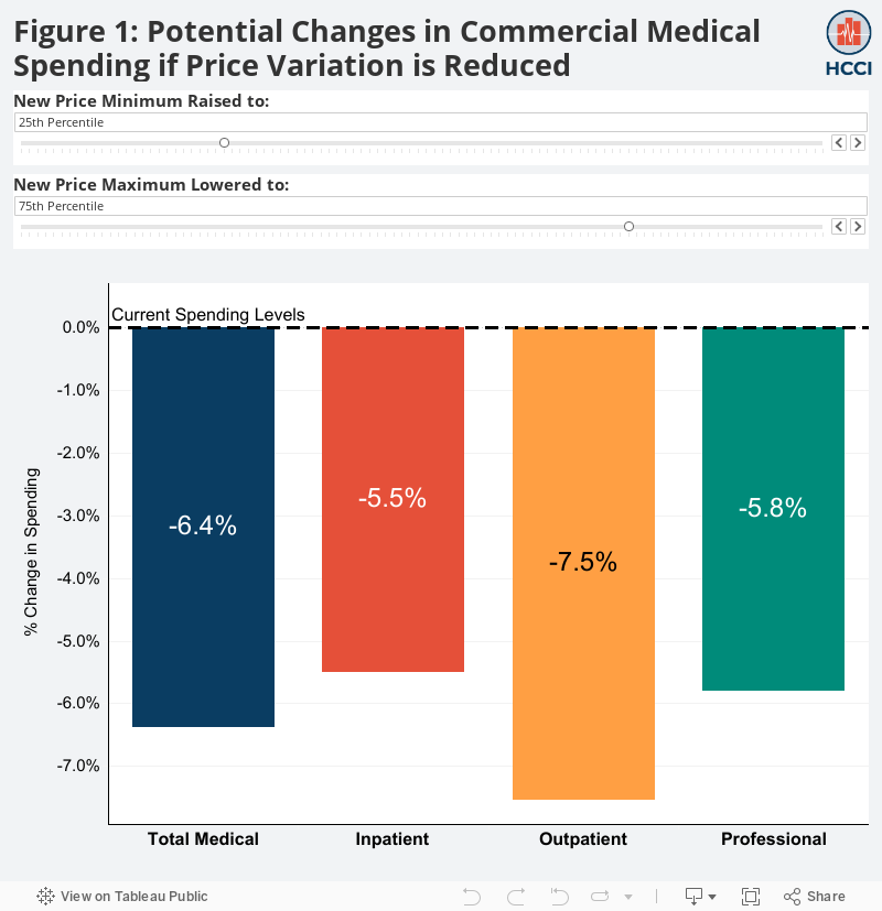
As the dashboard shows, different hypothetical combinations of the opposing reductions in price variation would lead to different effects on overall spending, holding all other factors constant. For instance:
- If the highest market prices – for each service – declined such that they were equivalent to the 60th percentile price today, spending would decrease even if the lowest-priced claims within all services were raised to the 59th percentile price;
- If the lowest 33% of prices – for each service –
increased to the 33rd percentile, spending would increase even if
the highest 10% of prices – for each service – were lowered to the 90th
percentile;
- If within each service, the highest-priced claims were lowered to the 75th percentile market price and the lowest-priced claims increased to the 25th percentile market price, spending would decline by 6.4%, and;
- Spending would increase overall if the lowest half of prices all increased to their service’s median market price and the uppermost quarter of every service’s prices declined to the 75th percentile.
How we Calculated the Potential Effects of Reducing Price Variation
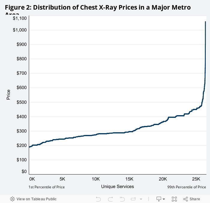
To understand our findings, consider an example of a single service in a single market: a 2-view chest X-ray in a major metropolitan area. The graph below displays the distribution and subsequent variation of a sample of those X-ray prices, ranked from least to most expensive left to right (Figure 2).We can calculate total spending on this service by adding the cost of each X-ray claim provided in the given area, displayed below as the area under the price line ($8.22 million in 2017).
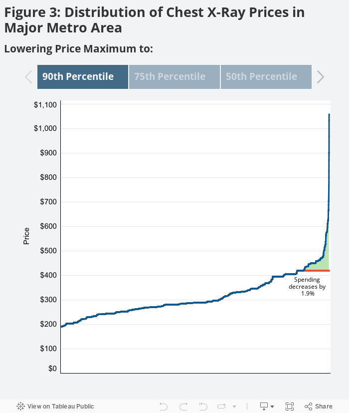
To see how a reduction in price variation might impact total spending on this service, we re-assigned the prices of all claims above (or below) a given price to that selected price. For example, consider if price variation were reduced by lowering the prices of the top 10% of X-ray claims. In this case, for all claims with prices higher than the 90th percentile, the 90th percentile price was assigned. Holding service use constant, the change in the market’s spending on 2-view chest X-rays would be equal to the sum of the price changes (the difference between the actual price paid and the selected price threshold) across all reassigned claims. Graphically, this is represented by the shaded area in green between the actual (blue) and the adjusted (orange) price lines (see Figure 3A).
Clicking through the graphs below, we see that the market’s spending on 2-view chest X-rays would decline 1.9%, 5.6%, and 13.6% if the prices for claims above the 90th percentile price (3A), the 75th percentile price (3B), and the median price (3C) were assigned to those threshold maximums, respectively.
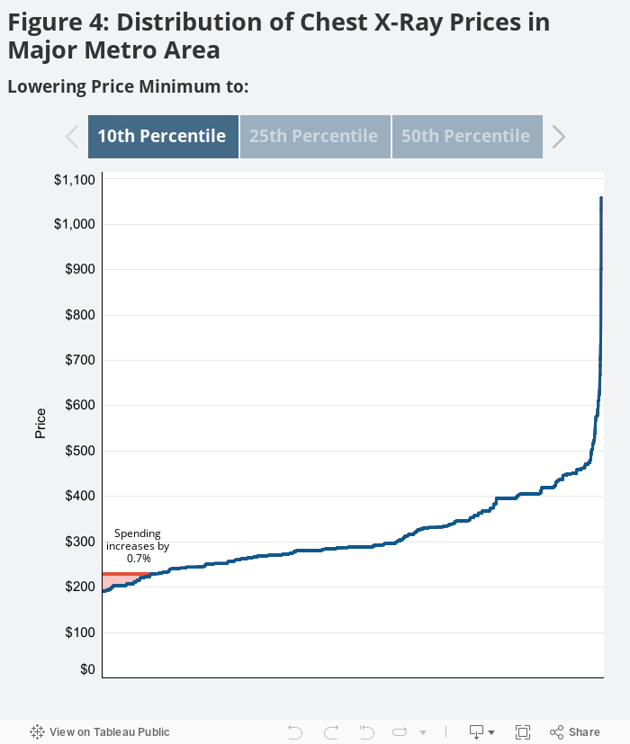
Conversely, if price variation were reduced by raising only the lowest-priced claims for this service to a given threshold, the market’s spending on this service would increase. Clicking through the arrows in the graph below – which explores the same sample price distribution for a 2-view chest X-ray in the same major metro area – one can see how much spending on this service would increase if the lowest-priced claims were reassigned to the new percentile price minimums. Similar to the previous graph, the sum of all price increases across all reassigned claims equates to the change in the market’s X-ray spending.
As displayed via the shaded area in red between the adjusted (orange) and actual (blue) price lines, spending in this market on this service would increase by 0.7%, 1.9%, and 5.8% if the prices for claims below the 10th percentile price (4A), the 25th percentile price (4B), and the median price (4C) were adjusted to those new threshold minimums, respectively.
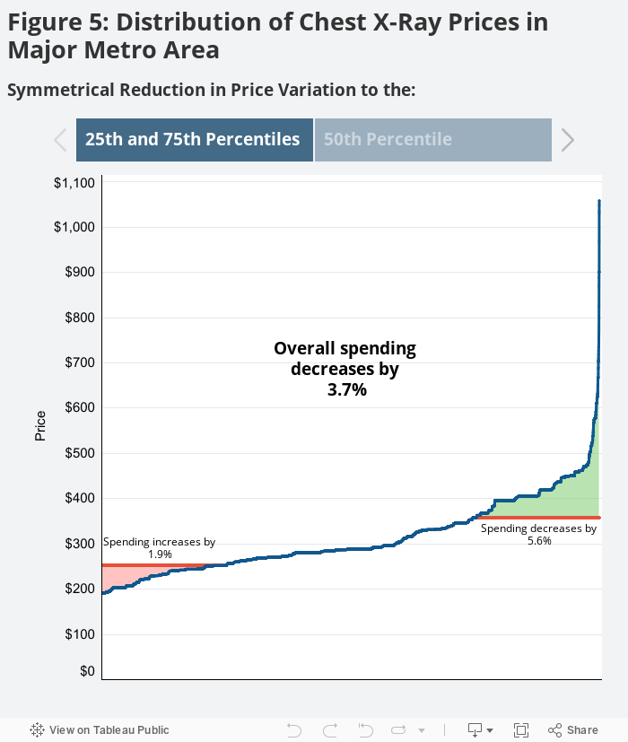
Price variation could also be reduced in both directions (adjusting high- and low-priced claims) simultaneously. In that case, the shape of a service’s price distribution in a given market in combination with the magnitude of the competing reductions in variation would determine what happens to spending. Consider the same sample of 2-view chest X-ray prices in the same major metro area as before. The distribution is skewed to the right, suggesting that a symmetric reduction in price variation would result in a decline in spending on that service in that market, assuming use remained unchanged. We can see this decline in spending graphically below, as the area shaded green (representing the potential decline in spending) is larger than the area shaded red (the potential increase in spending) when price variation is reduced by an equal magnitude in both directions.
The first view in the graph below shows the impact on the market’s X-ray spending if the price variation was reduced by raising the lowest-priced claims to the 25th percentile price and lowering the highest-priced claims to the 75th percentile price (Figure 5A). The second view (5B) shows the impact on the market’s X-ray spending if price variation was reduced by applying the median market price to all claims. Clicking through both examples, we see that market spending on this service would decline 3.7% and 7.7% if price variation were reduced to the 25th and 75th percentile scenario and reduced to the median price scenario, respectively.
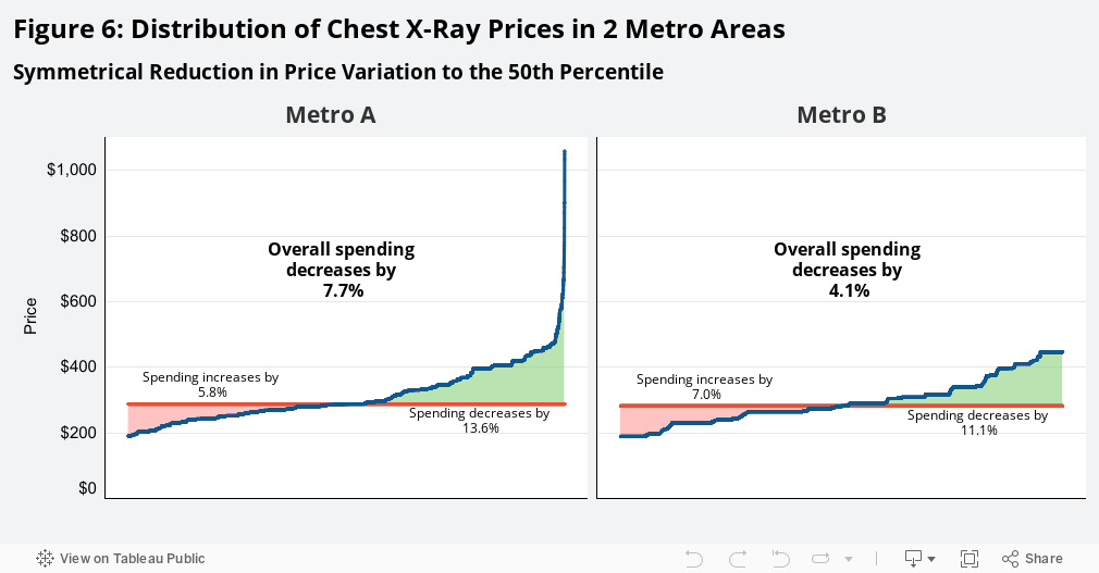
Furthermore, two metro areas with differently-shaped price distributions would experience different changes in their spending on a given service even if the reductions in price variation were similar in magnitude across the two geographies. Take, for instance, a sample distribution of 2-view chest X-ray prices within a second major metro area (“Metro B”). Metro B has a more evenly distributed set of X-ray prices, and therefore the same reductions in its price variation would have different effects on spending compared to the previous metro area (“Metro A”). This is shown in Figure 6 when we apply the median market price to all claims within each market. While the potential decrease in Metro B’s X-ray spending (shaded green) is larger than its potential increase in spending, the more even price distribution mitigates that decline in spending. Spending in Metro A would decrease 7.7%, while spending in Metro B would decrease 4.1%. The differences in these distributions help explain how the reduction in price variation can have varying effects on spending by service and by market.
If Price Variation Were Only Reduced in One Direction, Nationwide
Using the methods outlined above, we calculated the hypothetical effects that each potential reduction in price variation might have on medical spending at the national level for our sample population. Similar to the way we calculated adjusted spending on 2-view chest X-rays in a major metro area under a select set of example adjustments to price variation, we calculated adjusted spending for all percentile price adjustments, both individual and in combination, for all services in a market. For each percentile(s) adjustment to price variation, we summed the adjusted service spending levels across all services within a market. Those total adjusted market spending levels were summed across all markets to find the effect that each potential price variation reduction had on national spending.
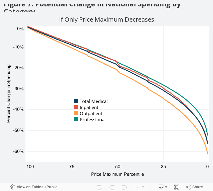
When examining all services across the country, we found that the more price variation was reduced from the higher-priced side of the distribution, the greater the decline in national medical spending. For each service, if the price of the lowest-priced claim was applied to all of that given service’s claims within all markets, spending would be cut by more than half (-56%) nationwide. If the highest-priced half of claims – within each service – were lowered to their service’s median market price, spending would decline by 19%. Interestingly, if the prices of the highest-priced claims fell only to the 90th percentile of prices for their service, spending would still decline by almost 4%.
As the shape of price distributions can vary by service and market, we explored whether this one-sided reduction in price variation would lead to different effects on medical spending by category of service. While the potential effects were largely similar across categories, we found there would be a slightly greater decline in outpatient spending compared to professional spending, and the difference increased as the reduction in variation from the high-priced end became more severe. This suggests the distribution of outpatient prices tended to skew more toward higher prices compared to the distribution of professional service prices.
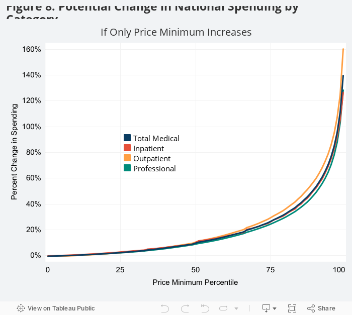
On the other hand, the greater the reduction in price variation that occurred as a result of upward pressure on the lowest-priced claims, the more medical spending for our sample would increase across the country. If the highest market price for each service was applied to all claims within each service, spending would increase nearly 2.5-fold (+140%) nationwide. However, the majority of that increase would come from the most extreme reduction in price variation (i.e., the uppermost group of high prices being applied to all claims). If the cost of the lowest-priced claims increased to the 10th percentile price within each service, commercial medical spending would go up less than 1% across the country. Furthermore, if the lowest-priced half of claims increased to their service’s median market price, spending would increase 10.1%. There was very little variation in potential effects of one-sided upward reduction in price variation on spending by category of service.
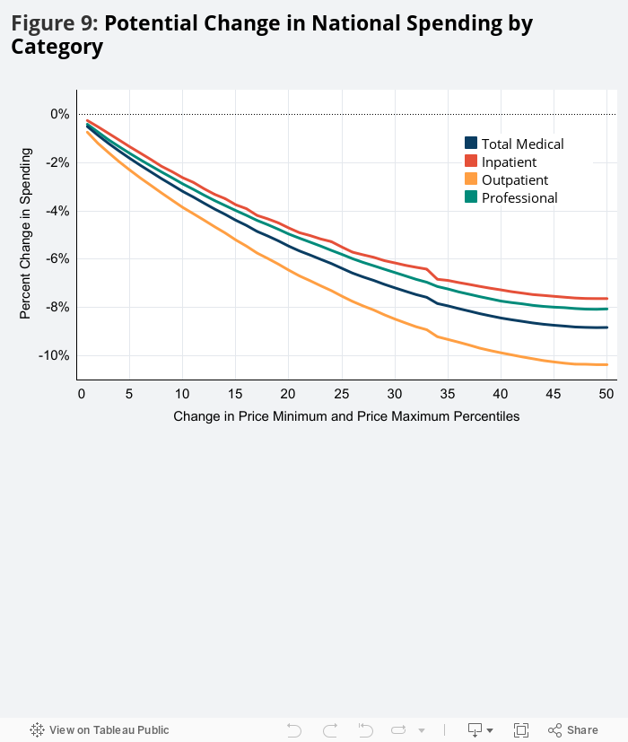
If Price Variation Symmetrically Reduced from Both Directions, Nationwide
Possibly the most interesting scenario might be that price variation would not be reduced through increases in the price minimum or declines in the price maximum in isolation. But in fact, that the opposing reductions in the variation would occur simultaneously in both directions. As seen in the 2-view chest X-ray example, both the size of the reductions in variation in each direction and the shape of the given service’s price distribution determine the potential effect on total spending. To explore this, we tested what might happen to our sample’s medical spending if there were symmetrical reductions in price variation with the minimum and maximum prices being adjusted up and down to an equal degree.
Shown below in Figure 9, every balanced reduction in price variation resulted in a decline in spending nationwide. If the smallest potential change in prices occurred (i.e., the lowest-priced claims were raised to their given service’s 1st percentile market price and the highest-priced claims were lowered to their given service’s 99th percentile market price) medical spending would fall by 0.5%. If the largest potential balanced adjustment in prices occurred (i.e., the median rate was applied to all claims within all services in all markets), spending would decline by nearly 9%. This implies that the gap between highest-priced services and the median price is larger than the gap between the lowest-priced services and median. In other words, the distributions of prices tended to be skewed toward higher prices. As a result, these findings suggest that if there were a symmetric reduction in price variation in each market, assuming use stays constant, spending would go down.
Most of the potential decline in spending from the balanced reduction in prices came in the upper- and lowermost 20th percentiles. If within each service, the highest-priced claims were lowered to the 80th percentile market price and the lowest-priced claims increased to the 20th percentile market price, spending would decline by 5.4% – which is more than half of the potential effect that simply assigning median market prices to all claims had on national spending.
The balanced potential reductions in price variation are only meant to serve as interpretable examples. Use the interactive dashboard at the top of the article to explore what might happen to spending nationwide if price variation were reduced by any number of adjustments to the price minimum and/or the price maximum.
Limitations
To date, there are limited data and case studies analyzing how price transparency could affect U.S. health care prices and spending. This report is meant to serve as an example, powered by real data, of the potential effects a reduction in price variation – one of the stated goals of the new price transparency proposed rule – could have on medical spending. It is not meant to make definitive or predictive statements about the effect of any price transparency effort– even the one being proposed by the 3 agencies, which is one way among many other ways to reach some level of price transparency. The report simply attempts to use HCCI data to give context to a complex policy conversation often based on abstract theory or markets that do not necessarily act in the same manner as the U.S. health care industry. As such, the report has a number of limitations.
First, the adjusted spending numbers do not take into account how potential changes in price may affect utilization. Theoretically, lowering prices may entice more patients to use services, thus cancelling out any savings. Or, conversely, raising prices could lead to a decline in use. Relatedly, the study does not allow for potential substitution of newly lower- or higher-priced services.
Another limitation is that the analysis only focuses on potential price changes from the ends of the price distribution. It does not study whether there may be price shifts in the middle. For example, the prices between the 20th and 29th percentile may all raise to the 30th percentile, while no change happens to the prices between the 1st and 19th percentiles. While shifts like these are certainly plausible, this study does not account for the nearly enumerable number of potential reductions in variation.
The way in which we define and treat markets leads to additional limitations as a CBSA does not perfectly capture all health care markets. The analysis would not capture providers in two geographically proximate CBSAs that may compete over the same group of patients via their prices. Conversely, in larger CBSAs, the analysis may assume that providers are competing when they are not in reality (i.e., two hospitals in Manhattan and Long Island).
Furthermore, the study presumes that each service and each market will experience the same change in price variation. However, there are many reasons to suggest this may not be the case. For instance, two markets with different levels of provider and insurer market power could experience very different reductions in price variation both in magnitude and direction. It would be less likely for price variation to be reduced by lowering the highest-priced claims in metro areas where, for example, a provider had a large share of the market – an occurrence that is becoming more frequent as provider markets become more concentrated over time. It would similarly be less likely for price variation to be reduced by an increase in the lowest-priced claims in an area where an issuer had a large share of the market. Variation in other factors, such as network adequacy standards, “most favored nation” clauses, anti-tiering or anti-steering practices, or “all or nothing” contracts, could also result in different reductions in price variation (if at all) across markets. As such, treating all markets equally may over- or understate the potential effects of changes in price variation from market to market accordingly.
This study, however, is not intended to estimate the impact of the proposed policy as it does not predict both the extent and direction that price variation may be reduced (if at all). It is designed, simply, to contribute to the discussion of what may happen if price variation were reduced in any number of ways.
Methods Note
We analyzed a sample of 420 million commercial medical claims from the Health Care Cost Institute (HCCI) for the year 2017. Included claims had to be associated with a member who was under the age of 65, had an identifiable gender in the data, and had ESI, non-individual coverage with one of the following plan types: Health Maintenance Organization, Preferred Provider Organization, Point of Service Plan, or Exclusive Provider Organization.
We defined a claim as all claim lines for an individual with common dates and services codes (designated by DRG for inpatient claims and a CPT and CPT modifier combination for outpatient and professional claims). The allowed amounts for all claim lines within a given claim were summed, giving the price (or negotiated rate) for that specific claim. The sum of all the prices for a given service within a given market was defined as spending on that service in that market. Markets were defined at the core-based statistical area (CBSA) level – as defined by the U.S. Census Bureau. In total, claims from 963 CBSAs were analyzed.
We applied distinct inclusion-exclusion criteria that aligned with the methodology from the 2018-2019 Healthy Marketplace Index (HMI). For greater detail, see section 1.3 Claim Inclusion Criteria from the 2018-2019 HMI Technical Appendix. In total, the sample used in this report made up 61% of total medical spending and 78% of total medical use within HCCI’s 2017 commercial claims database.
For a given service-market combination, the prices for all claims were ranked to determine the prices for the 1st through 99th percentiles. Prices above or below were adjusted to match the selected percentile price, and then prices were summed again to find the adjusted spending on the service within the market depending on the desired minimum or maximum threshold effect. This analysis was performed for every service, within every market, for every potential (combination of) percentile adjustment(s). The adjusted service-market spending amounts were then summed across all services within the market and across all markets to calculate adjusted spending nationwide. The adjusted spending was compared to the unadjusted spending to determine the potential effects of each reduction in price variation.